Xynk Quick Tour
Some of the basic features and capabilities of Xynk illustrated with a built-in example file.
- Example Files
- The Xynk Main Window
- Graphing
- ANOVA results
- Post-Hoc Symbols
- Exporting Results
- Where to go from here
Example Files
Select the File -> Examples menu to open the example file "2-way ANOVA 2 Levels".
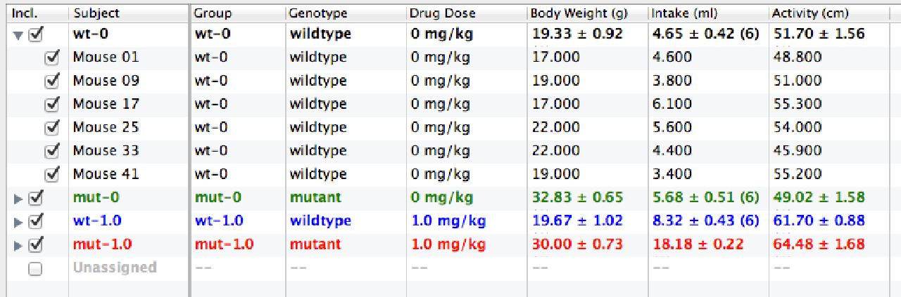
This file contains an artificial data set of 24 subjects divided into 4 groups, with 3 independent categorical measures: "Group", "Genotype" and "Drug Dose", and 3 dependent numeric measures: "Body Weight", "Intake", and "Activity". The data set simulates the effects of 2 different drug doses on either wildtype or mutant mice.
Other example files are also artificial to demonstrate different analysis set ups; or the files are standard datasets for validation of statistical routines. Some of the files are real-life behavioral data, too.
The Xynk Main Window
The file opens in the main Xynk window. There are 4 views or panes within the main Xynk Window: the data table, the measures list, the groups list, the current graph, and the graph caption.

The Data Table shows the individual category assignments and data points for each subject. The data is initially shown in a grouped, folding view of the data (with group means).
You can change the table format by toggling the "Data View" button in the tool bar:

Now the data table displays a flat, ungrouped view of all the subject data:

By clicking on the check boxes, you can include or exclude subjects or entire groups from graphing and analysis.
The Measures List shows the data set's categorical measures, tagged with a "c", and its numeric measures tagged with a "#" badge. Unchecking a measure both hides its column in the data table and excludes.
The Groups List lets you quickly exclude or include groups from the analysis.
The Graph View graphs a subset of the data with the y-axis value specified by a numeric measure and with categorical measures along the x axis. Pop-up menus for choosing the graph X and Y measures are below the caption.
The Caption beneath the graph displays the statistical analysis of the current graph.
Graphing
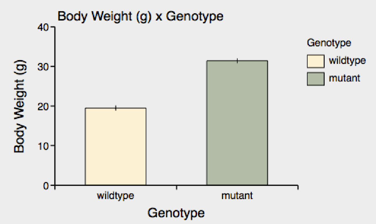
A Xynk graphs a dependent y-value measure at experimental categories within the data set. At the moment, the graph is displaying the "Body Weight" of mice against the "Genotype" category.

You can change the y-value in 2 ways:
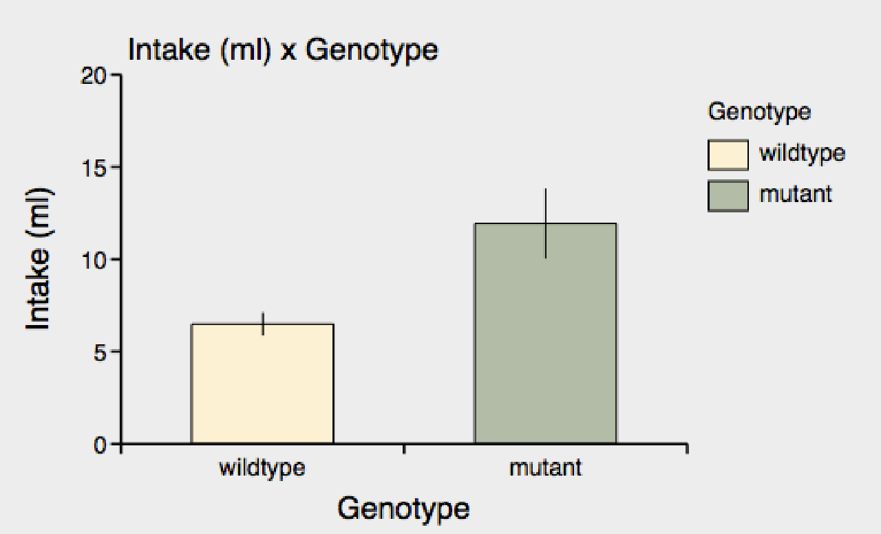
1) You can click on a different numeric measure (#) in the list of measures to the left of the graph view. For example, we can click on "# Intake" measure in the list of measures, to graph "Intake" by "Genotype"

2) You can select a numeric measure from the y-value pop-up menu underneath the graph. For example, selecting "Activity" to graph "Activity" by "Genotype".


You can change the x-axis category from the category pop-up menu under the graph, or by option-clicking on a category measure in the measure window. For example, selecting X-Category: "Drug Dose" to graph "Intake" by "Drug Dose".


You can reverse the order of categories on the x-axis using the reverse button next to the category popup:
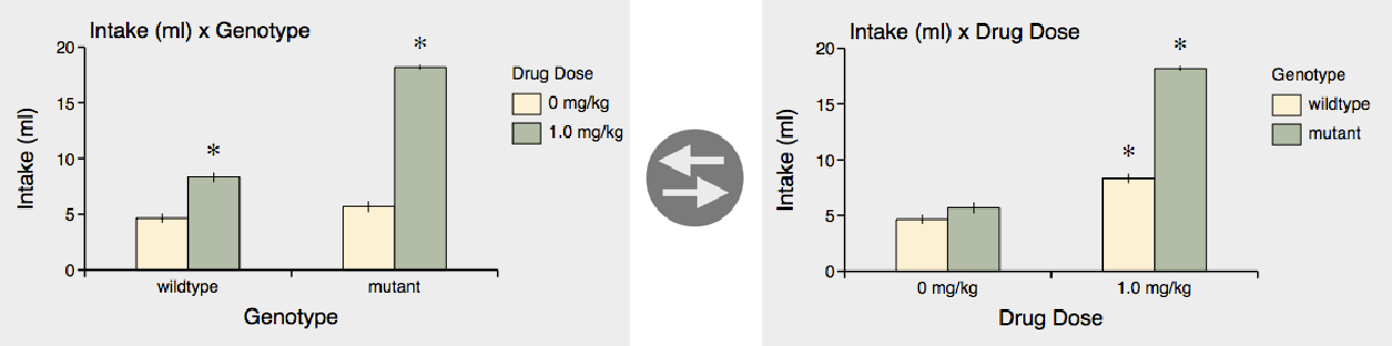
You can also specify a subcategory with the subcategory pop-up menu, to plot a subset of bars within each main category. For example, selecting "Genotype" as the subcategory will plot "Intake" with "Genotype" bars within each "Drug Dose" main category.
(The subcategory also has a reverse button that reverses the order of subcategories.)


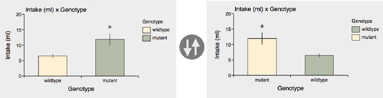
A really convenient feature is that you can easily swap the category and subcategory using the swap button.
You can quickly view the individual data points that contribute to the graph by toggling between showing the means and showing all individuals via the "Pts/Means" tool bar button.

ANOVA results
Xynk automatically calculates 1-way and 2-way ANOVAs when categorical and numeric measures are selected for graphing, if the data allows. A summary of the ANOVA results is shown in the caption under the graph.
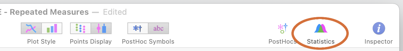
For more detailed results, click on the Statistics button in the tool bar to show the Statistics window.
The current numeric and categorical measures are shown at the top and can be changed via the pop-up menus.
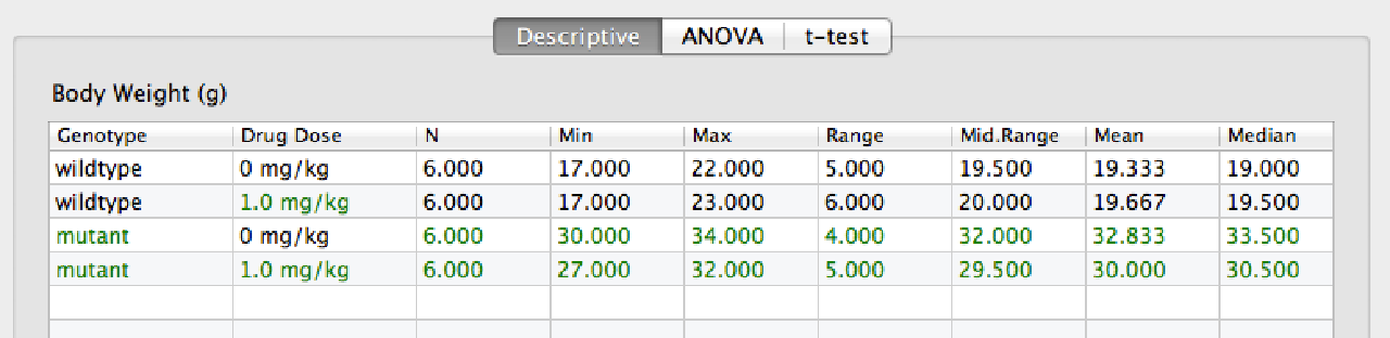
The Descriptive tab shows the summary statistics for the current y-value measure for each cell of the current graph (i.e. for each combination of category and subcategory).
The ANOVA tab shows the full ANOVA table, and a table of all the post-hoc comparisons.
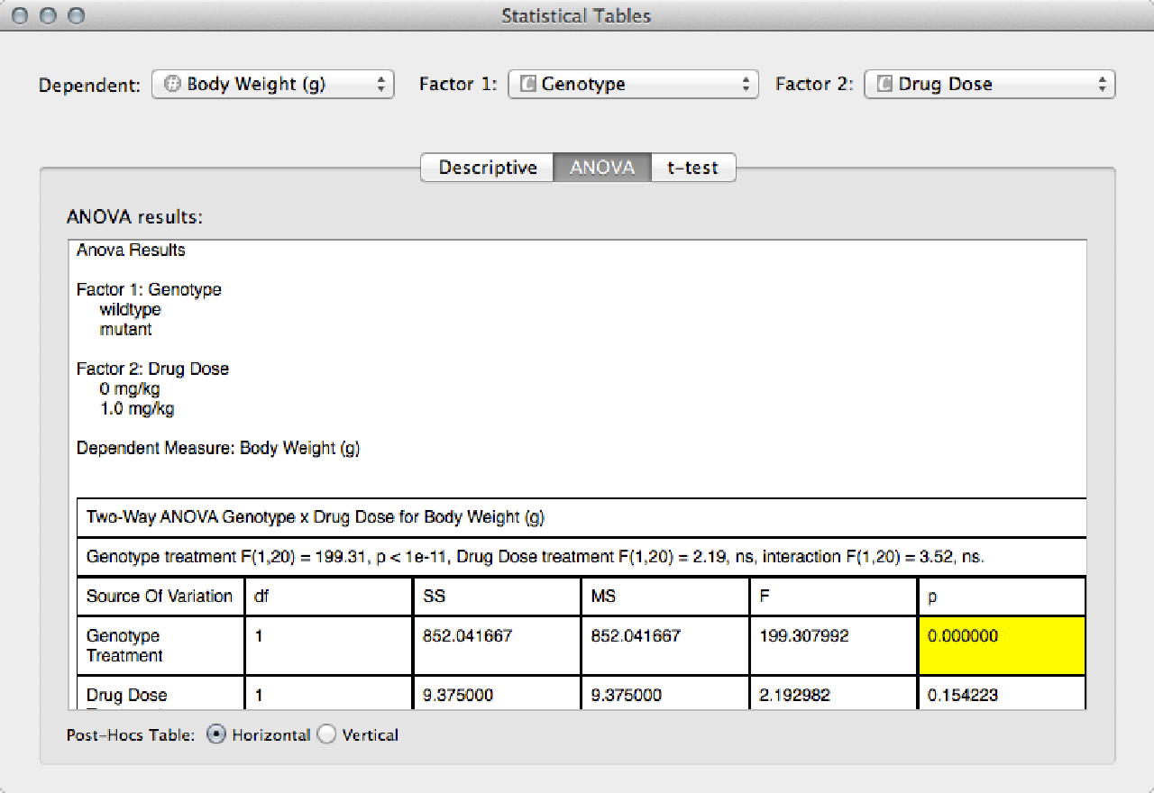
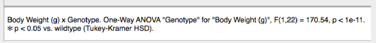
Significant differences (p < 0.05) are highlighted.

If you change the dependent measure or the categorical factors, the ANOVA is automatically recalculated.
Underneath the ANOVA results table, all possible post-hoc comparisons are shown.
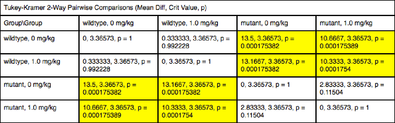
Note that you can toggle the post-hoc comparions between either a "horizontal" display or a "vertical" display.

The vertical post-hoc display:

Post-Hoc Symbols
If the ANOVA results are significant, Xynk can show post-hoc results directly on the graph. Post-hoc results can be specified in 2 ways:
1) specific post-hoc differences can be shown with an asterix or other symbol by setting up post-hoc comparisons. You can edit post-hoc comparisons by clicking on the PostHocs button.
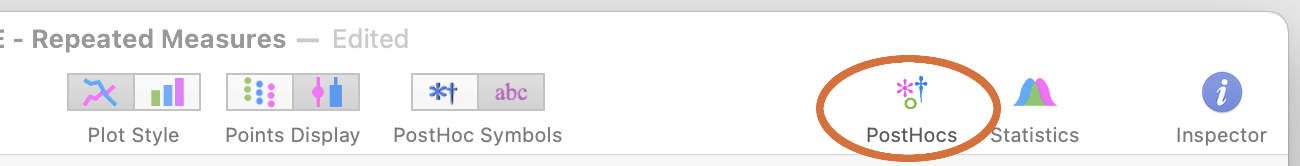
This brings up the post-hoc comparions window. Add a new post-hoc comparison by clicking on the "+" button. For each comparison, you specify a post-hoc symbol (such as * or †), and which groups should be labeled if significantly different from the comparison group.

In the first comparison, groups are labeled if different from the "0 mg/kg" Drug Dose group within the same Genotype. This comparison will be tested and labeled across all graphs displaying these groups, even if you switch y-values.
With this post-hoc comparison, asterices are placed above the "1.0 mg/kg" groups of both wildtype and mutant mice.

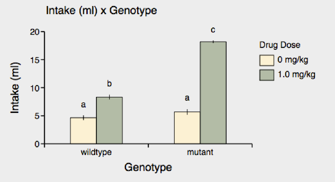
2) Alternatively, you can show all post-hoc differences and label significantly different groups with different letters. Just click on the "abc" button of "PostHocLabels".

Letters appear above each bar; bars with different letters are significantly different. Now you can see that while the "0 mg/kg" groups are not significantly different from each other, both "1 mg/kg" groups are different from the "0 mg/kg" groups and from each other.
Exporting Results
To export the statistical results, you can select,copy and paste the caption text.
The graph can be copied or saved as a PDF image, and then placed in a document or presentation. (You can also option-click on the graph, and then drag-and-drop it into another document.)
Where to go from here
Importing Data coming soon
Graphing Parameters coming soon
Repeated Measures coming soon